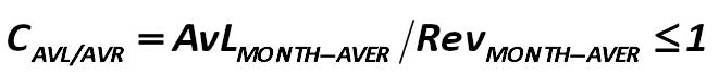
For example, assuming that the ratio of the average value of liabilities to be paid to the average value of sales revenue (CAVL/AVR) must be less than 1: Alexander Shemetev
2-37.jpg:661x68, 8k
|
|
|
|
For example, assuming that the ratio of the average value of liabilities to be paid to the average value of sales revenue (CAVL/AVR) must be less than 1: Alexander Shemetev 2-37.jpg:661x68, 8k |
 And at the atomic approach – the calculation of covariance is reduced to: Such prominent scientists are the followers of this approach as: Y.R. Magnus, P.K. Katishev, A.A. Presetskiy 2-54.jpg:738x155, 12k |
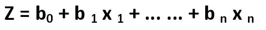 Classically, the equation of linear discriminant analysis is recorded in the same form in which it was opened by Edward Altman: Ronald Aylmer Fisher 233.jpg:547x62, 5k |
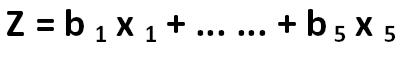 Edward Altman proposed a regression equation whose general form is: Edward Altman 234.jpg:419x57, 4k |
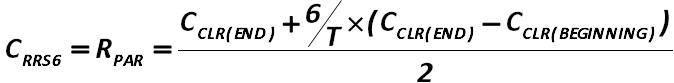 When the poor balance sheet structure is found – it is necessary to verify the real possibility of the company to restore its solvency; it is made by the ratio-to- restore-the-solvency (RRS6) calculation for a period of 6 months: Alexander Shemetev 235.jpg:674x83, 9k |
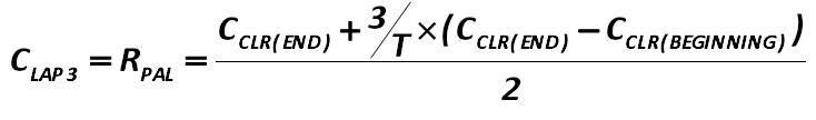 If the value of the coefficient shows less than 1, it is necessary to calculate the rate-of-loss-of-ability-to-pay (LAP3): Alexander Shemetev 235_1.jpg:734x108, 10k |
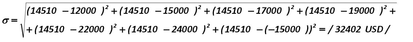
 For example, assuming that the ratio of the average value of liabilities to be paid to the average value of sales revenue (CAVL/AVR) must be less than 1: Alexander Shemetev 236.jpg:661x68, 8k |
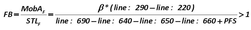 The ratio of the presence of signs of fraudulent bankruptcy can be calculated by the algorithm: Alexander Shemetev 237.jpg:876x106, 15k |
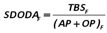 The first indicator is security of the debtor’s obligations to creditors by debtor’s assets (SDODA): Alexander Shemetev 238.jpg:372x118, 6k |
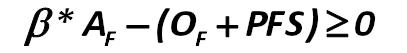 The third indicator is the inequality of the secured obligations by net assets, which is not strictly fixed by the legislator: Alexander Shemetev 239.jpg:407x53, 4k |
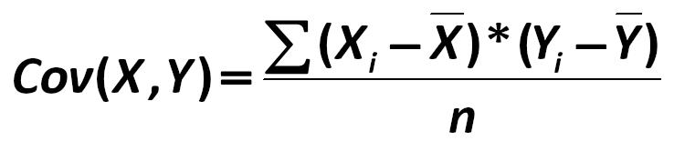
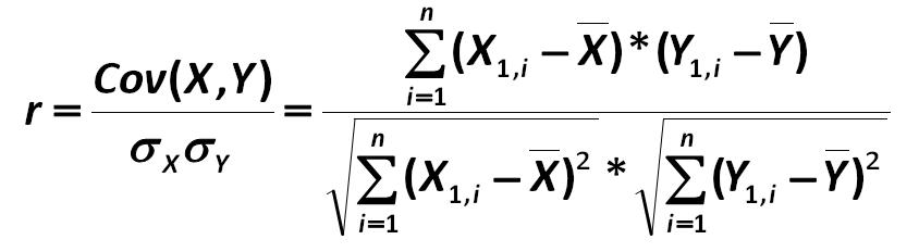 Correlation (r) – is expressed mathematically by a linear 1 relationship between two variables . It is calculated by the formula: Sir Francis Galton 240.jpg:844x232, 21k |
 It should be noted that: Sir Francis Galton 241.jpg:360x159, 7k |
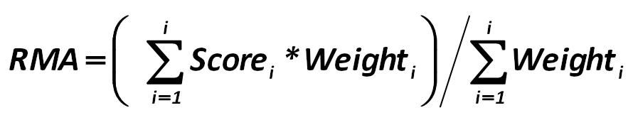
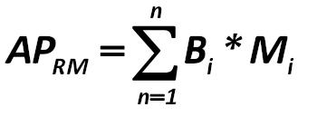 This is how the average probability of return in the market calculation looks like (APRM): Karl Pearson 242.jpg:350x129, 5k |
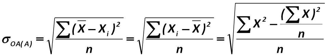
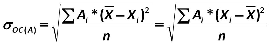
 The classical approach to the analysis of variations: Saint-Petersburg State University of Economics and Finance, for example, L.S. Tarasevich, P.I. Grebennikov, A.I. Leussky 243.jpg:663x93, 9k |
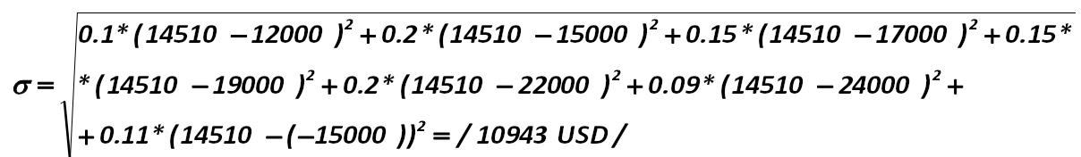
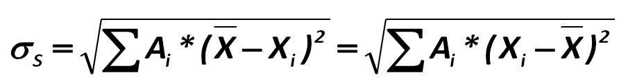 However, if you want to estimate the most probable value of the deviation (rather than the total scale as it is in the calculation of (?)), then use a standard measure of standard deviation (SigmaS): Saint-Petersburg State University of Economics and Finance, for example, L.S. Tarasevich, P.I. Grebennikov, A.I. Leussky 244.jpg:905x122, 13k |
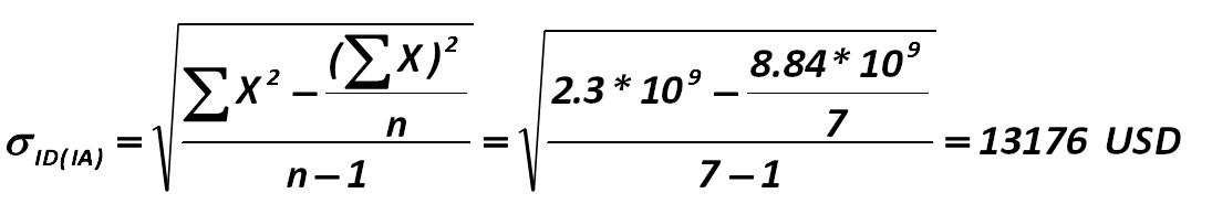
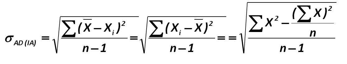 The classical school of information-atomic approach involves the following calculation of the absolute standard deviation: Prominent advocates of this approach to the analysis are the John E. Hanke, Artur G. Reitsch, Dean W. Wichern, V.P. Nosco (Moscow State University), K. Dougerti, A. Aivazian, V. Mkhitaryan and others. 245.jpg:1115x208, 22k |
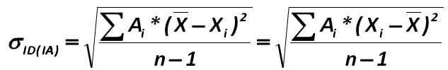 The weighting approach for the information-atomic school includes: Prominent advocates of this approach to the analysis are the John E. Hanke, Artur G. Reitsch, Dean W. Wichern, V.P. Nosco (Moscow State University), K. Dougerti, A. Aivazian, V. Mkhitaryan and others. 247.jpg:633x99, 10k |
 The classical approach involves the calculation of the absolute standard deviation from the formula: Such prominent scientists are the followers of this approach as: Y.R. Magnus, P.K. Katishev, A.A. Presetskiy. 248.jpg:1100x189, 20k |
 Along with the classic, there is the weight sub-atomic approach within this school, which requires the calculation of standard deviation: Such prominent scientists are the followers of this approach as: Y.R. Magnus, P.K. Katishev, A.A. Presetskiy 249.jpg:949x172, 18k |
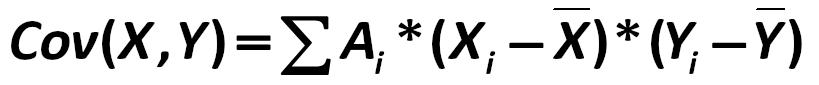 Covariance at a weight variational approach is equal to: Saint-Petersburg State University of Economics and Finance, for example, L.S. Tarasevich, P.I. Grebennikov, A.I. Leussky 250.jpg:819x85, 11k |
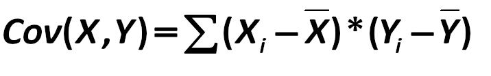 Or, if you use the classic variational approach, it is: Saint-Petersburg State University of Economics and Finance, for example, L.S. Tarasevich, P.I. Grebennikov, A.I. Leussky 251.jpg:716x112, 10k |
 In the information-atomic approach, the covariance is calculated as follows: Prominent advocates of this approach to the analysis are the John E. Hanke, Artur G. Reitsch, Dean W. Wichern, V.P. Nosco (Moscow State University), K. Dougerti, A. Aivazian, V. Mkhitaryan and others. 252.jpg:742x164, 13k |
 And at the atomic approach – the calculation of covariance is reduced to: Such prominent scientists are the followers of this approach as: Y.R. Magnus, P.K. Katishev, A.A. Presetskiy 253.jpg:738x155, 12k |
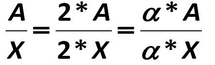 The similarity of this ratio is defined by the following properties of fractions: Akhmim wooden tablets or Cairo wooden tablets, 2-nd - 3-rd millenium BC 254.jpg:442x135, 10k |
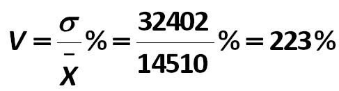
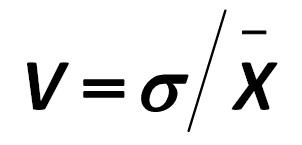 If the value of standard deviation (o) is to be divided by the most-likely- probability of the profit margin, we obtain a coefficient of variation: Sir Francis Galton 255.jpg:302x145, 4k |
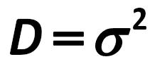 The calculations often use the variance (D or ? ) / theoretical value of the scatter of the values /, which is the standard deviation in the square: Sir Francis Galton, Karl Pearson 256.jpg:211x91, 3k |
|
Sometimes, when there are some more complex calculations, for example, the portfolio planning, you want to calculate the amount of variance of two variables, which is equal to: Harry Markowitz 257.jpg:955x76, 12k |
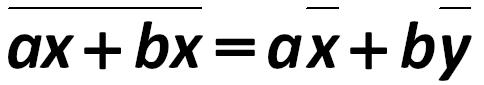 Also important is the decomposition formula for the sum of two average- means: Harry Markowitz 258.jpg:484x85, 8k |
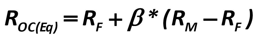 Then, under these model conditions, the next formula is working: William F. Sharpe 259.jpg:905x147, 14k |
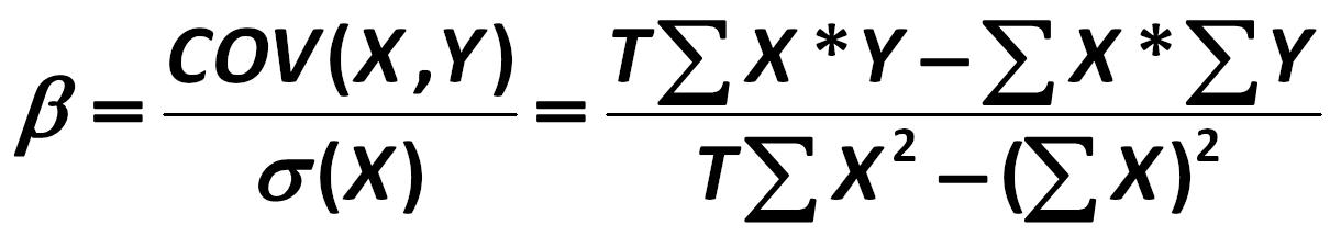 The ? coefficient is calculated on the basis of statistical data. In this case, we consider a stock market for a relatively long period. Then, the ? coefficient is calculated as follows: William F. Sharpe 260.jpg:1210x215, 32k |
 Then the expected yield of the portfolio is: Stephen Alan Ross 261.jpg:1360x131, 18k |
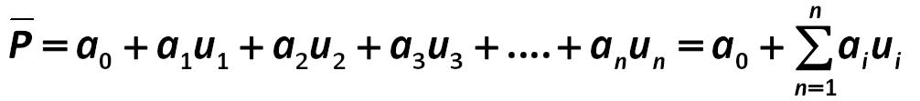 So, we know the average portfolio yield. According to the model of APT, the expected return ( P) is given by (261): Stephen Alan Ross 261a.jpg:1006x111, 12k |
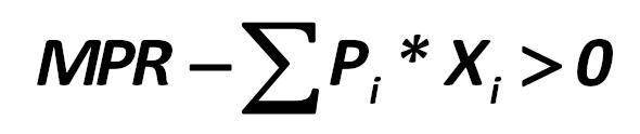 Portfolio, dependent on one single factor, with the appearance of the arbitrage securities’ party can be optimal if: Stephen Alan Ross 262.jpg:590x124, 8k |
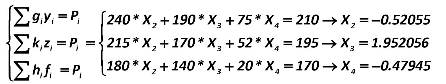
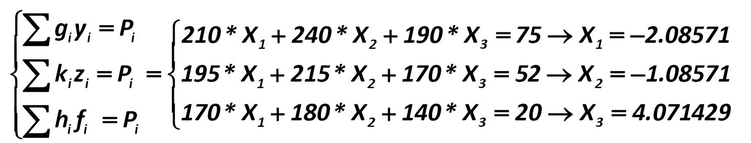
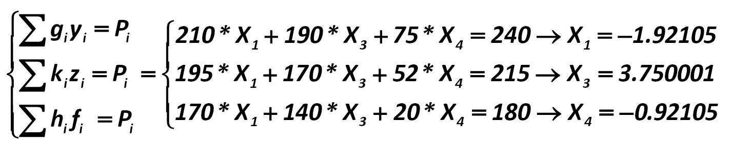
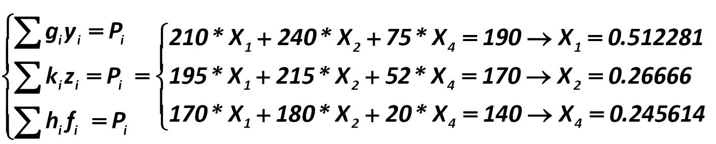
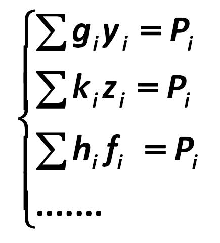 Xi is calculated from the equations: Stephen Alan Ross 263.jpg:435x479, 18k |
|
Thus, the optimal portfolio 1 (OP) with the choice of asset portfolio as a privileged one should be constructed as follows: Alexander Shemetev 264.jpg:988x64, 12k |
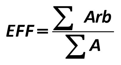 The effect of arbitrageurs is calculated as follows: Stephen Alan Ross 265.jpg:407x218, 9k |
 Since the CAPM model is used, this multiplier appears in the system of equations, which takes the form: Stephen Alan Ross 266.jpg:1196x529, 53k |
 Sensitivity to changes in the EXR for the old portfolio will be: Stephen Alan Ross 267.jpg:891x81, 11k |
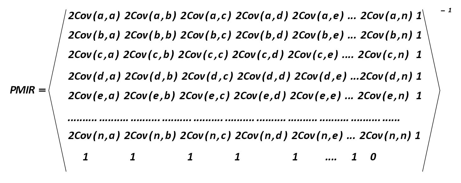 The formula for calculation of the portfolio with minimal risk (PMIR) is as follows (268): Harry Markowitz 268.jpg:1467x583, 101k |
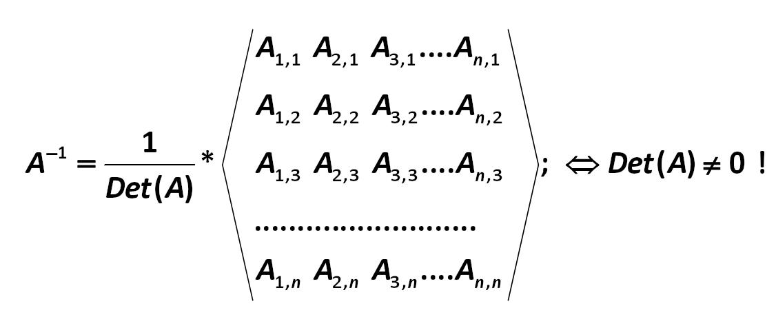 The formula for calculating the inverse matrix (А ) is as follows: Gauss-Jordan 269.jpg:1126x460, 33k |
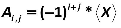 А1,1; А2,2; ….; Аn,n – is the matrix, the derivatives of the first by means of decomposition. Decomposition is: Gauss-Jordan 270.jpg:412x97, 5k |
|
Profitability of such portfolio is given by: Harry Markowitz 271.jpg:1120x71, 14k |
 A portfolio risk is defined as: Harry Markowitz 272.jpg:1011x87, 12k |
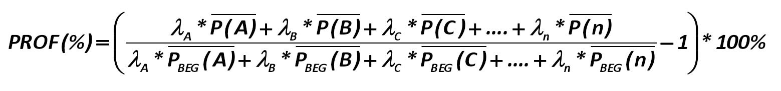 So, how to calculate a yield? Portfolio yield/profitability (PROF(%)) with minimal risk is (273): Alexander Shemetev 273.jpg:1559x182, 35k |
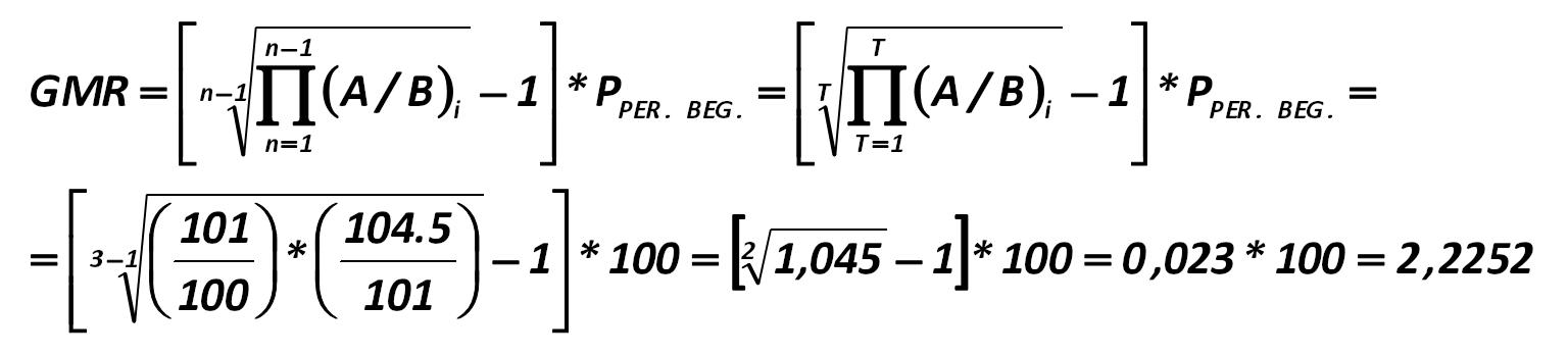
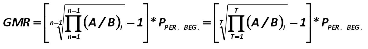 The general formula for calculating the geometric middling return is: Harry Markowitz 274.jpg:1222x165, 22k |
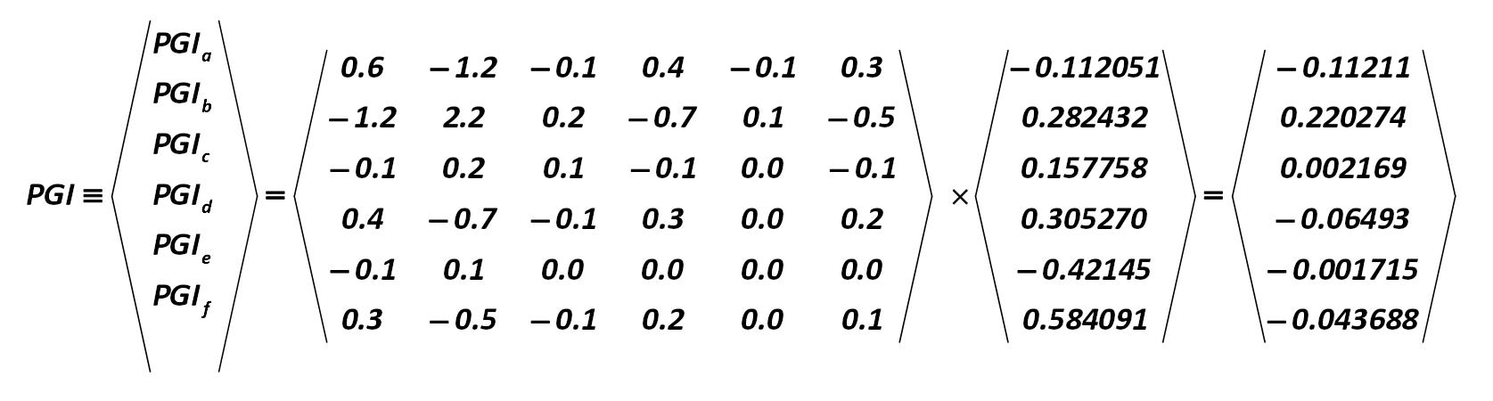
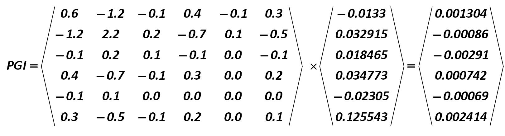
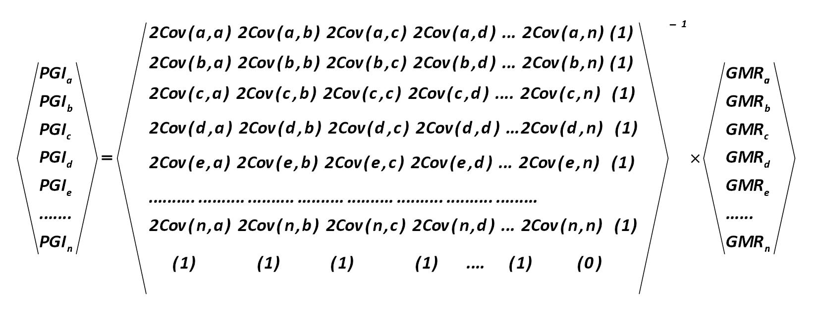 Portfolio with a given income (PGI) is calculated from the matrix multiplication (275): Harry Markowitz 275.jpg:1647x653, 112k |
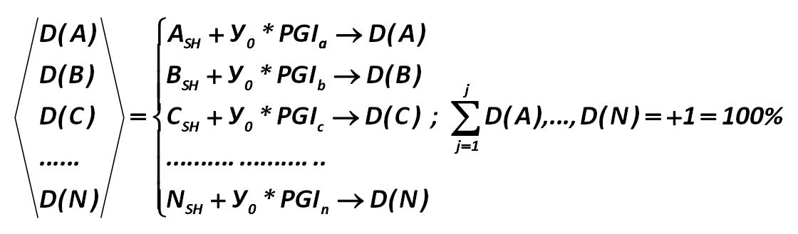 Thus, the data array can be calculated manually or by computer. This array will allow us to find answers to the equation more easily that will allow us to calculate the constants in your optimal portfolio. Harry Markowitz 276.jpg:1120x329, 36k |
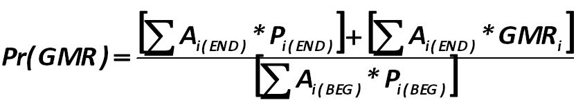 The geometric average return on the portfolio with minimal risk (Pr(GMR)) will be 2.37494%.This value is calculated from the formula: Harry Markowitz 277.jpg:845x155, 17k |
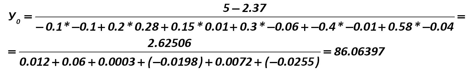
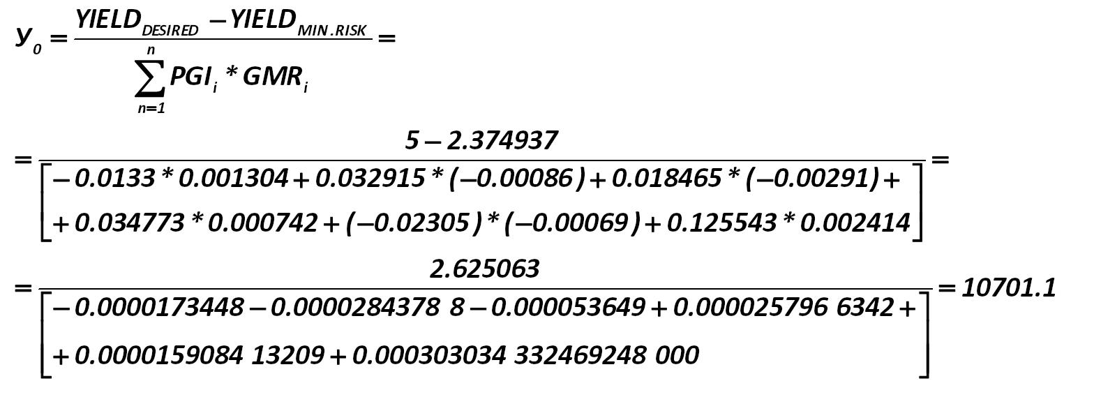
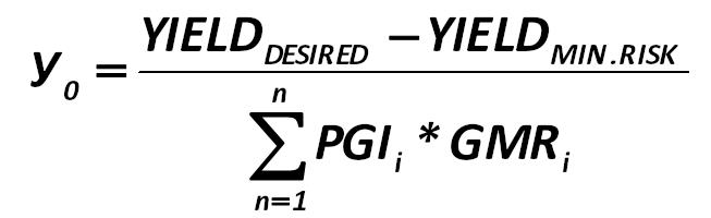 Only the Y0 index remained unknown to us from the optimal portfolio, which is calculated by the formula: Harry Markowitz 278.jpg:653x200, 14k |
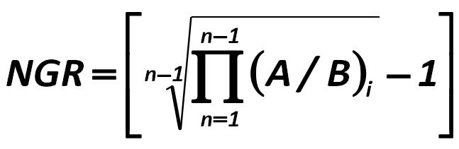 Alexander Shemetev offers to calculate the nominal geometric return (NGR). To calculate this index, you must first calculate the total geometric earnings per share as follows: Harry Markowitz 279.jpg:647x211, 13k |
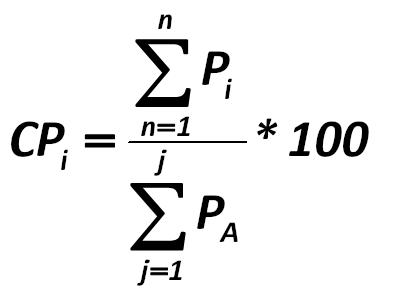 hen the available for the period of observation actual fluctuations in the price of securities must be brought into the conditional price (CP) as follows: Alexander Shemetev 280.jpg:403x300, 10k |
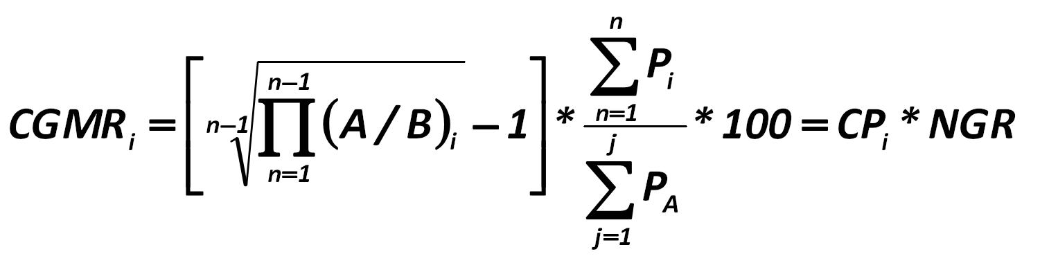 Under these conditions, the author of this paper believes rational to expect the conditional geometric middling return (CGMR), which is calculated using the method developed by Alexander Shemetev on the basis of the following formula (281): Alexander Shemetev 281.jpg:1527x380, 36k |
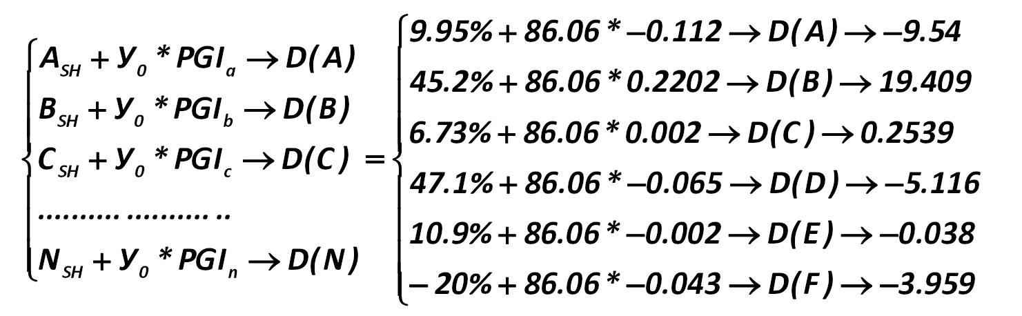
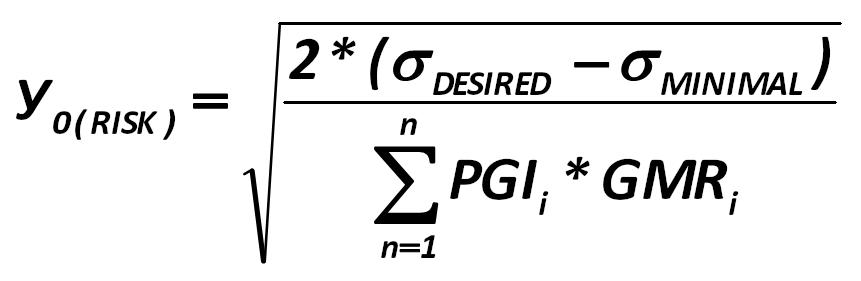 the optimal portfolio in terms of risk an investor can create by creating a new system of equations by means of indicator Y0 (risk): Harry Markowitz 282.jpg:861x281, 23k |
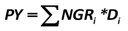 Target cell must become Portfolio’s Yield (PY), which is equal to the sum of products of geometric middling of returns per share for the period (NGRi) and the share of each security in the portfolio (Di): Harry Markowitz 283.jpg:518x128, 8k |
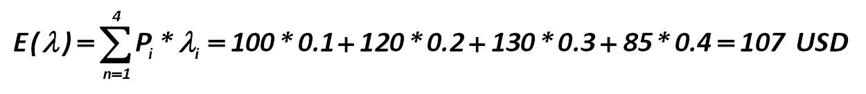
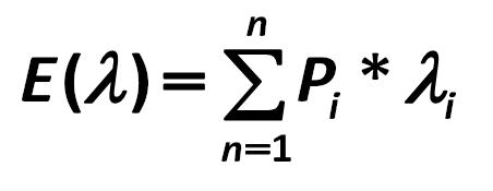 In mathematics, a similar calculation is called the mathematical expectation: Blaise Pascal 284.jpg:452x175, 7k |
 EVA is calculated as: Peter Drucker 2841.jpg:813x93, 12k |
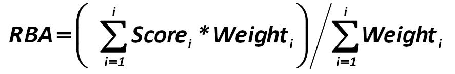 When scoring method: Alexander Shemetev 285.jpg:887x145, 16k |
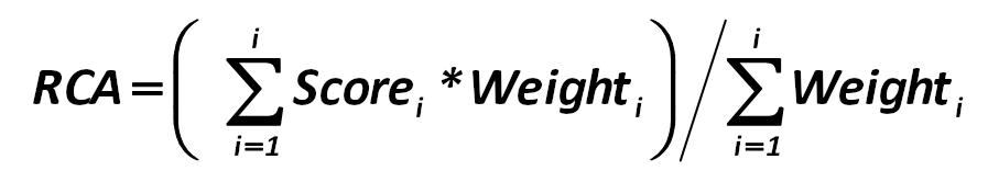 Calculation of capital quality and capital adequacy is conducted as follows: Alexander Shemetev 287.jpg:897x166, 15k |
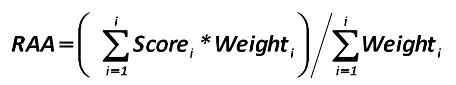 The calculation of the quality and sufficiency of the assets is held by the following formula: Alexander Shemetev 288.jpg:902x168, 16k |
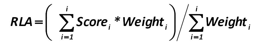 The calculation of the quality of the aggregation of property of company and the adequacy of its liquidity is held by the following formula: Alexander Shemetev 2881.jpg:902x168, 15k |
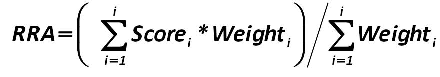 The calculation of the quality and adequacy of return is carried out by the formula: Alexander Shemetev 289.jpg:881x155, 16k |
 The calculation of the quality and adequacy of management is carried out by the formula: Alexander Shemetev 290.jpg:890x169, 16k |
 This is the simplest method. If you do not have time to apply the bulky models – this technique is the "compact" calculated by the formula (297): Edward Altman 297.jpg:970x138, 20k |
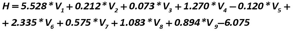 John Fulmer’s model divides the company to potential bankrupts and non- bankrupts. Coefficient V of J. Fulmer models is (299): John Fulmer 299.jpg:973x109, 19k |
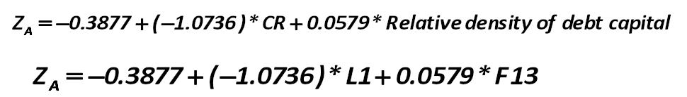
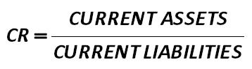 L1 (CR) - Current Ratio John Burr Williams 301.jpg:358x99, 7k |
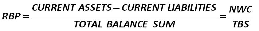 The method involves the calculation of the coefficient of bankruptcy prediction (RBP) by the formula: Russian Federation Government 305.jpg:843x104, 18k |
 Thus, the coverage ratio of current financial needs (CFN) is calculated by the formulas: E.S. Stoyanova 308.jpg:730x97, 12k |
|
O-H1 – is a figure equal to the ratio of net book value (NBV) to book value of assets (TBS): Silvia Horvathova and Pavol Olejnik 310.jpg:248x38, 3k |
|
O-H2 – is a measure of payback of debt, expressed in years: Silvia Horvathova and Pavol Olejnik 311.jpg:313x34, 3k |
|
O-H3 – is the ratio of net cash flow for the period (NCFP) to the carrying amount of production issued during the period (PDP). Silvia Horvathova and Pavol Olejnik 312.jpg:249x35, 3k |
|
O-H4 – is the ratio of operating profit to book value of assets (ROA, return on assets): Silvia Horvathova and Pavol Olejnik 313.jpg:231x39, 2k |
|
a linear discriminant model and its explanation for forecasting bankruptcy on the basis of the index of financial stability IFS (314): D. Baran, A. Palfy, Z. Chvancharova, P. Olejnik, S. Horvathova, K. Zalai, J. Shnircova, L. Kalafutova, P. Ruchkova, E. Kislingerova and other 314.jpg:699x42, 7k |
 The costs are calculated by the formula: Alexander Shemetev 4-47.jpg:290x160, 4k |
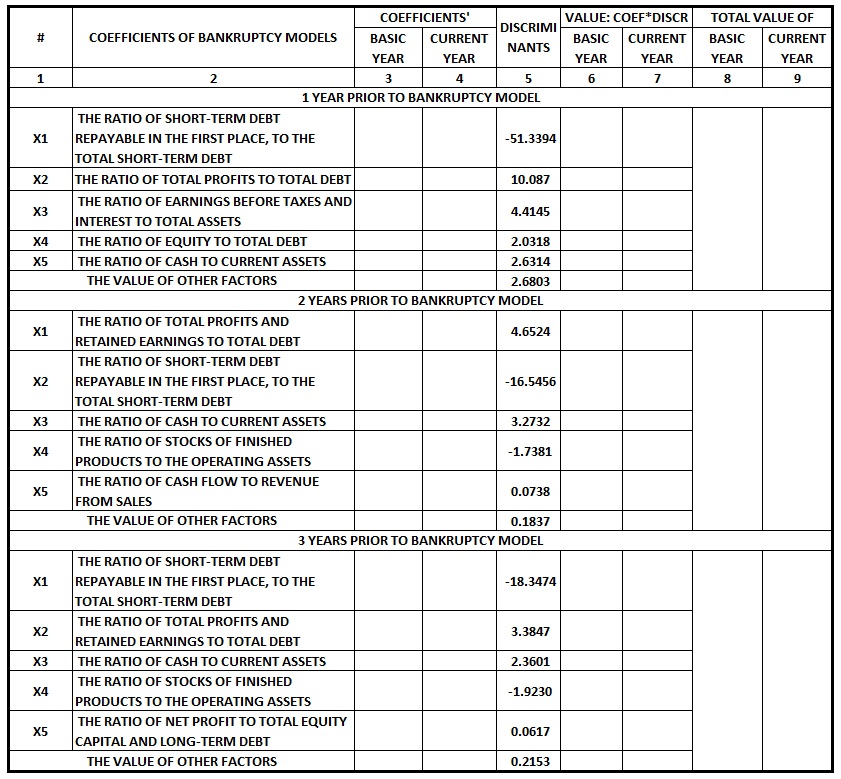
 So, I think you already understand: how to calculate the first stage of the model. Coefficients are calculated, then they are substituted into the linear discriminant model by using the following formula: Gibson-Stickney-Schroeder-Clark 414.jpg:1108x126, 20k |
 Further, the value of Y is substituted into the following minus-logit model: Gibson-Stickney-Schroeder-Clark 415.jpg:285x150, 4k |
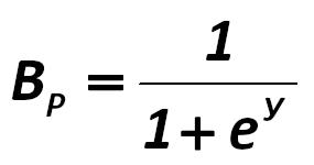
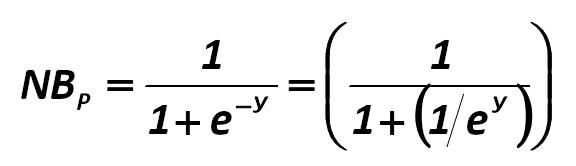 Accordingly, the logit analysis shows the probability that the company is not bankrupt (NBp): Gibson-Stickney-Schroeder-Clark 416.jpg:576x166, 9k |
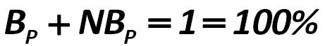 The amount of data of logit and minus-logit analysis should be equal to 1: Alexander Shemetev 417.jpg:461x66, 6k |
 For example, the volatility of the simplest security, part of an option, bond, is calculated by the formula: Black-Scholes-Merton 418.jpg:959x208, 25k |
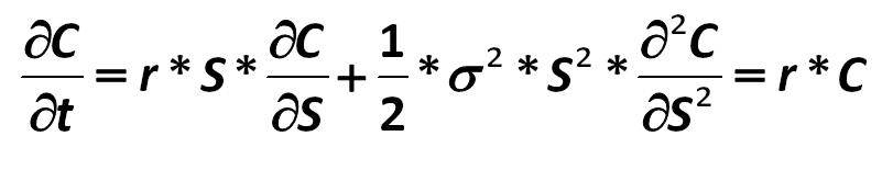 The differential equation of the Black-Scholes option involves optimization of the portfolio to minimize risk: Black-Scholes-Merton 419.jpg:811x155, 13k |
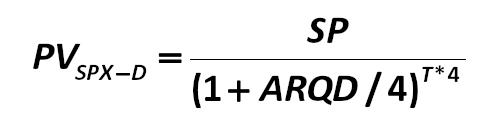 There is a need for some additional calculations to apply this formula. First, one must calculate (PVSPX– D) the present value (PV – Present Value) of Stock-Price in X-dividend condition (that is, Ex-dividends, that is, excluding the cost of dividends): Gibson-Stickney-Schroeder-Clark 420.jpg:489x119, 7k |
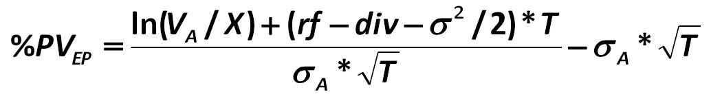
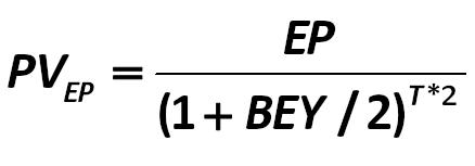 The second necessary component for the intermediate calculation is PVEP: present value of the exercise price (strike price): Gibson-Stickney-Schroeder-Clark 421.jpg:438x153, 7k |
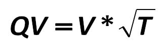 The third essential element is the cumulative rate volatility (QV): Gibson-Stickney-Schroeder-Clark 422.jpg:330x92, 4k |
|
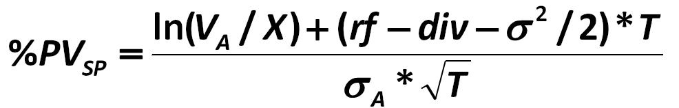
I think all of you have a table editor Excel. In this editor, 1 perform the following operations. To calculate the % PVSP : Gibson-Stickney-Schroeder-Clark 423.jpg:1071x56, 14k |
|
To calculate the% PVEP: Gibson-Stickney-Schroeder-Clark 424.jpg:1071x75, 13k |
 In accordance with the axiom of Merton, if we were making the calculation by methods of classical analysis, (%PVSP) would be equal to: Black-Scholes-Merton 425.jpg:986x158, 18k |
 A (%PVEP) would be equal to: Black-Scholes-Merton 426.jpg:1034x147, 16k |
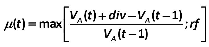 You also need to calculate the value of ? (t), which describes the expected market return from the options: Gibson-Stickney-Schroeder-Clark 427.jpg:734x168, 14k |
 The value of COV will be: Gibson-Stickney-Schroeder-Clark 428.jpg:920x86, 13k |
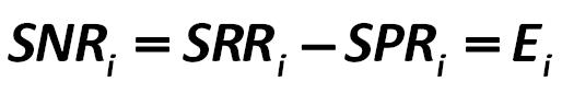 E, or SNR (Swap net rate): Robert Jensen 429.jpg:514x85, 7k |
 Professor R. Jensen’s method is based on the index of the nominal value of NCRP (Notional cash receivable / payable), which he recommends to be denoted as G: Robert Jensen 430.jpg:616x55, 7k |
 In order to assess what the company pays for the swap and the counterparty pays that – count rate L, which is equal to –PV: ED 162-B standard 431.jpg:250x86, 2k |
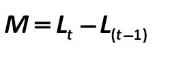 Positive or negative for the company amount payable to the recovery of the swap transactions will be calculated based on the index M: ED 162-B standard 432.jpg:252x86, 2k |
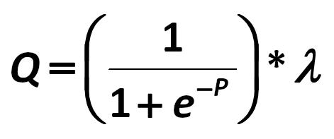 Q - is the total score of the model. Hatem Ben-Ameur, Bouafi Hind, Pierre Rostan, Raymond Theoret, Samir Trabelsi 433.jpg:471x197, 8k |
|
The index P is calculated by the formula (434): Hatem Ben-Ameur, Bouafi Hind, Pierre Rostan, Raymond Theoret, Samir Trabelsi 434.jpg:1373x67, 16k |
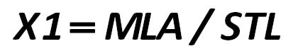 X1 - this is a quotient: the most liquid assets (MLA) to the sum of short- term borrowings (STL): Hatem Ben-Ameur, Bouafi Hind, Pierre Rostan, Raymond Theoret, Samir Trabelsi 435.jpg:413x79, 5k |
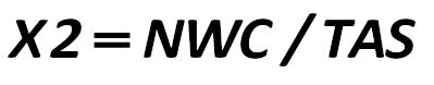 X2 - is the ratio: net working capital (NWC) to total assets (TAS): Hatem Ben-Ameur, Bouafi Hind, Pierre Rostan, Raymond Theoret, Samir Trabelsi 436.jpg:399x78, 5k |
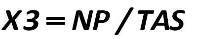 X3 - is the ratio: net income/profit (NP) to total assets (TAS): Hatem Ben-Ameur, Bouafi Hind, Pierre Rostan, Raymond Theoret, Samir Trabelsi 437.jpg:399x79, 6k |
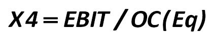 X4 – is the ratio of EBIT to capital (OC(Eq)). EBIT – as you remember – is the sum of operating income, interest expense and excessive interests in the Russian accounting. Hatem Ben-Ameur, Bouafi Hind, Pierre Rostan, Raymond Theoret, Samir Trabelsi 438.jpg:414x82, 6k |
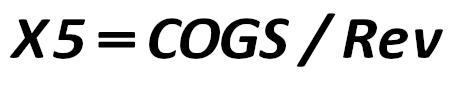 X5 – is the ratio of COGS to revenues (Rev). Hatem Ben-Ameur, Bouafi Hind, Pierre Rostan, Raymond Theoret, Samir Trabelsi 439.jpg:454x86, 7k |
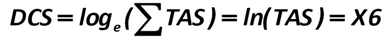 Discriminant company size (DCS) – is the natural logarithm of total assets of the company: Hatem Ben-Ameur, Bouafi Hind, Pierre Rostan, Raymond Theoret, Samir Trabelsi 440.jpg:796x86, 11k |
 The new Olson’s model versions: Harvard University version 2009/2010 Olson’s model versions: Harvard University version 441.jpg:468x144, 7k |
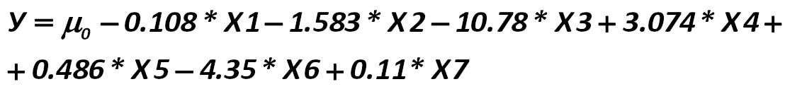
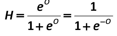
 In this model, e – is the familiar constant – the exponent (2.71828 ...). O – is the degree of the erection of the exponent. Indicator O is calculated by the formula (442): Olson’s model versions: Harvard University version 442.jpg:1314x117, 21k |
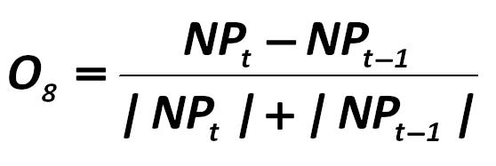 O8 is the figure calculated by the formula: Olson's model versions: Harvard University version 443.jpg:558x187, 11k |
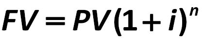 Our time period is greater than 1 year, investor, the parent company Co. Ltd. "Luck" considered advantageous profit interest calculations from the formula of compound interest: William George Horner 444.jpg:422x84, 5k |
 The costs are calculated by the formula: Alexander Shemetev 446.jpg:290x160, 4k |
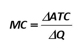
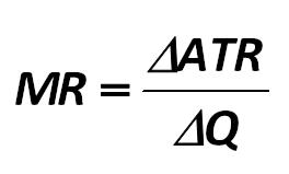 Marginal revenue is calculated as follows: Alexander Shemetev 447.jpg:264x159, 4k |
 The maximum profit will be achieved in the production of output, at which MR = MC, ie, the marginal cost equals to marginal revenue as it is shown in the formula below: 448.jpg:664x73, 10k |
 Net cash flow (NCF) consists of the following elements: 449.jpg:799x73, 10k |
|
long with the our direct and indirect method, some theorists, for example, N.Y. Gordo, secrete a liquid cash flow method, which involves the calculation by the formula: N.Y. Gordo 450.jpg:1054x75, 13k |
 Alexander Shemetev's photo Alexander Shemetev alexshemetev300dpi_2.jpg:300x301, 11k |
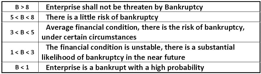 Table: The probability of bankruptcy by the Belarusian model G.V. Savitskaya belarusian_ratio.jpg:899x256, 56k |
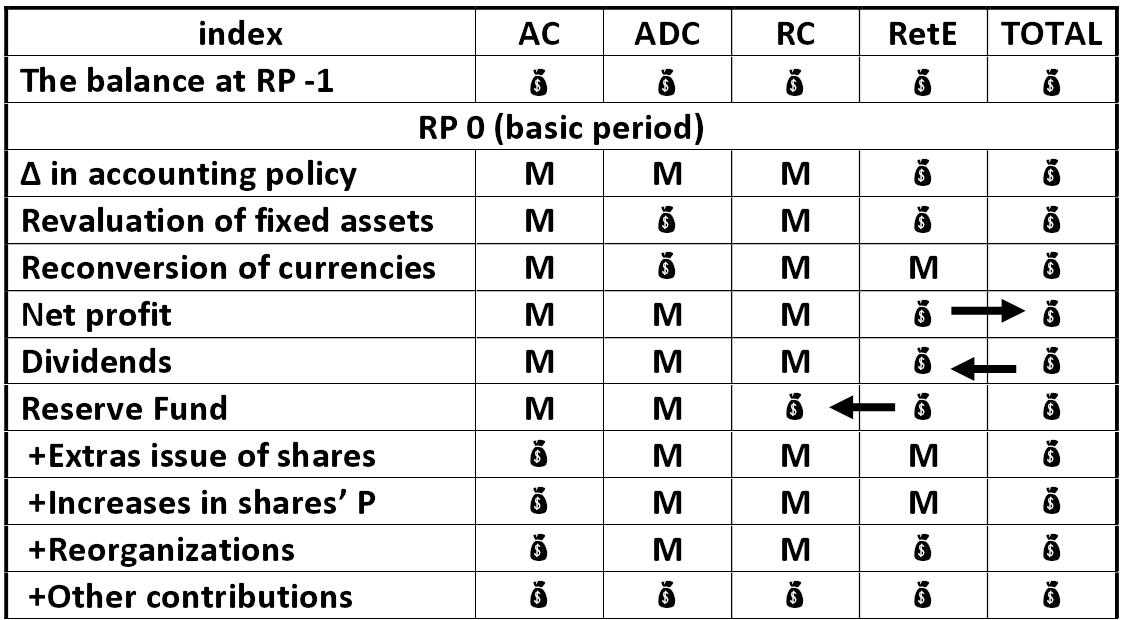 Scheme: Statement of changes in equity scheme Alexander Shemetev cap1.jpg:1125x620, 119k |
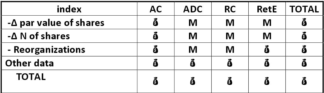 Scheme: Statement of changes in equity scheme Alexander Shemetev cap2.jpg:1118x322, 51k |
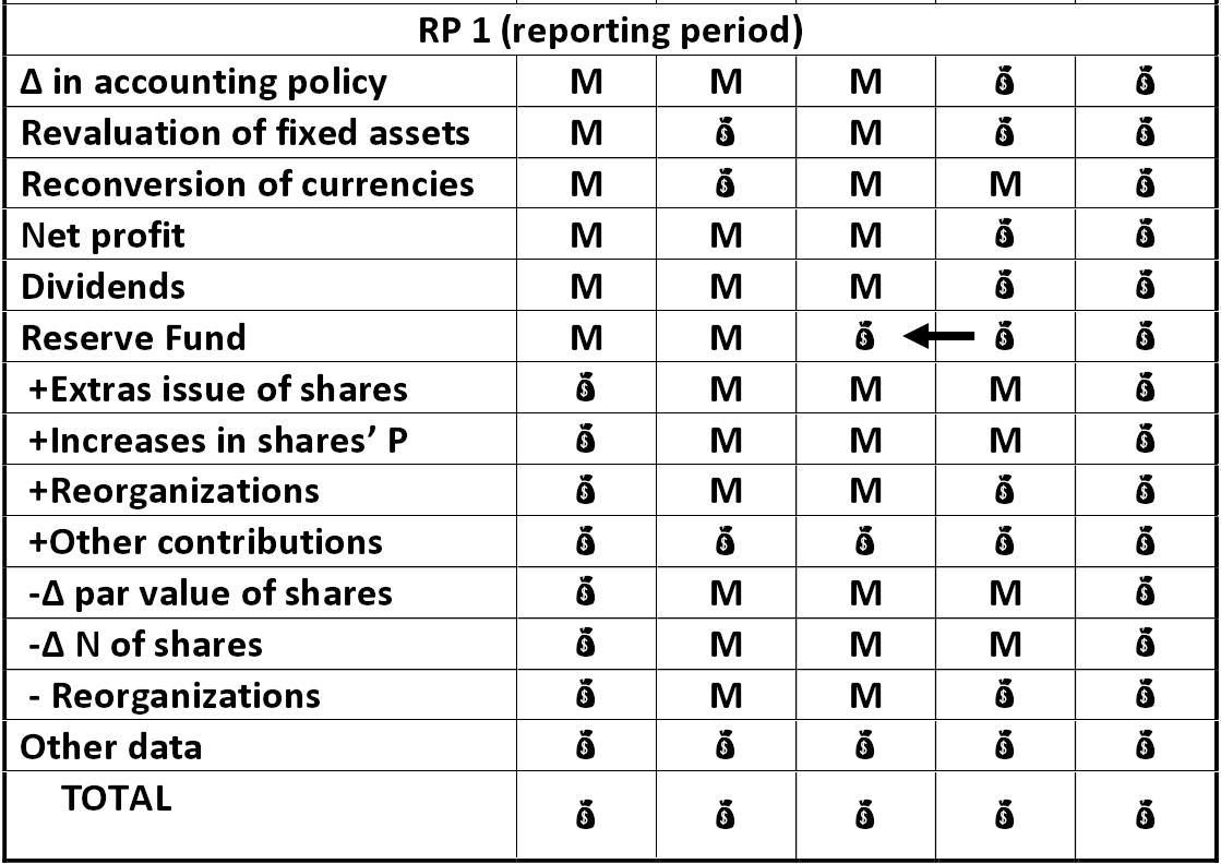 Scheme: Statement of changes in equity scheme Alexander Shemetev cap3.jpg:1119x792, 137k |
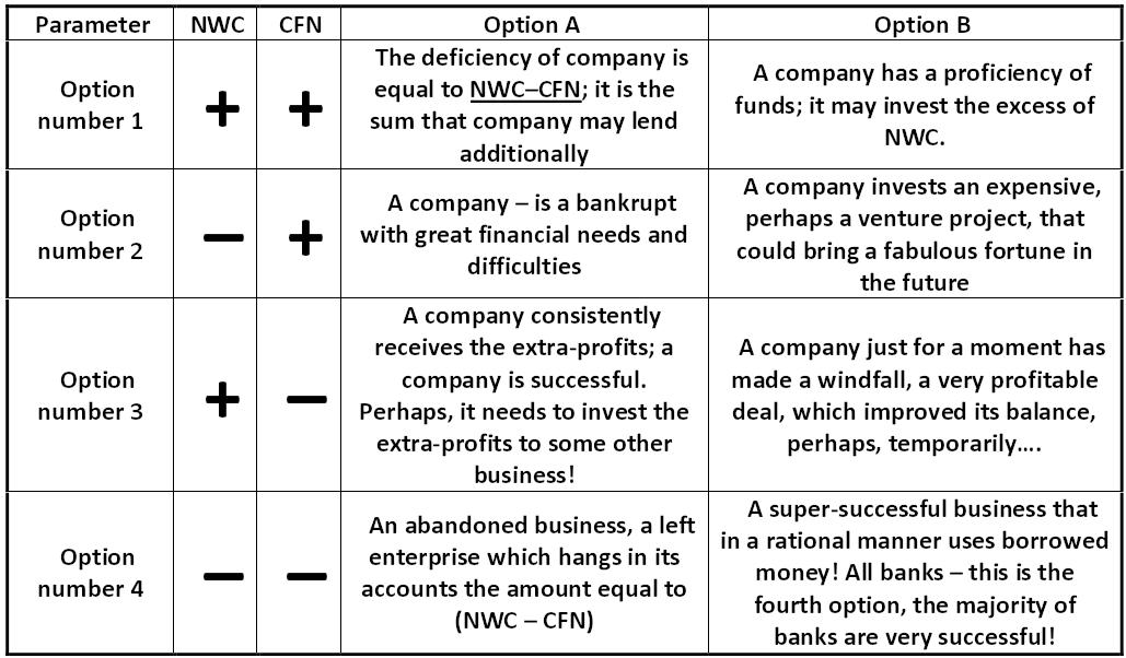 Table: Forecasting of bankruptcy by this method Alexander Shemetev cfntable.jpg:1029x602, 120k |
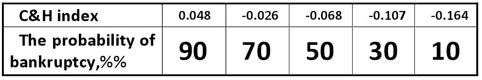 Table: Value of the C&H index Conan & Holder ch.jpg:991x166, 31k |
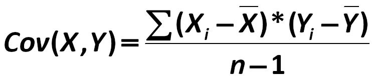
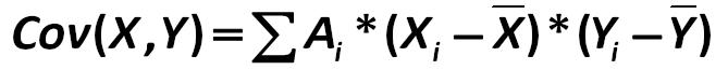 The covariance is calculated as follows: covcalc.jpg:669x78, 8k |
 So, if we optimize the portfolio by selling the asset number 1, then the company 1 has the opportunity to earn the following amount arbitrageurs : Alexander Shemetev e-6.jpg:1510x285, 54k |
 In this example, the risk for the company not to make a profit in each future period is most likely to be: Alexander Shemetev e1.jpg:1377x140, 30k |
 Optimal portfolio is determined by the formula (262): Alexander Shemetev e10.jpg:950x90, 12k |
 It is left only one global variant to compare this option with: portfolio optimization through the sale of the portfolio number 4. Alexander Shemetev e11.jpg:1486x284, 54k |
|
Arbitrageur of third option of portfolio optimization is: Alexander Shemetev e12.jpg:1357x97, 19k |
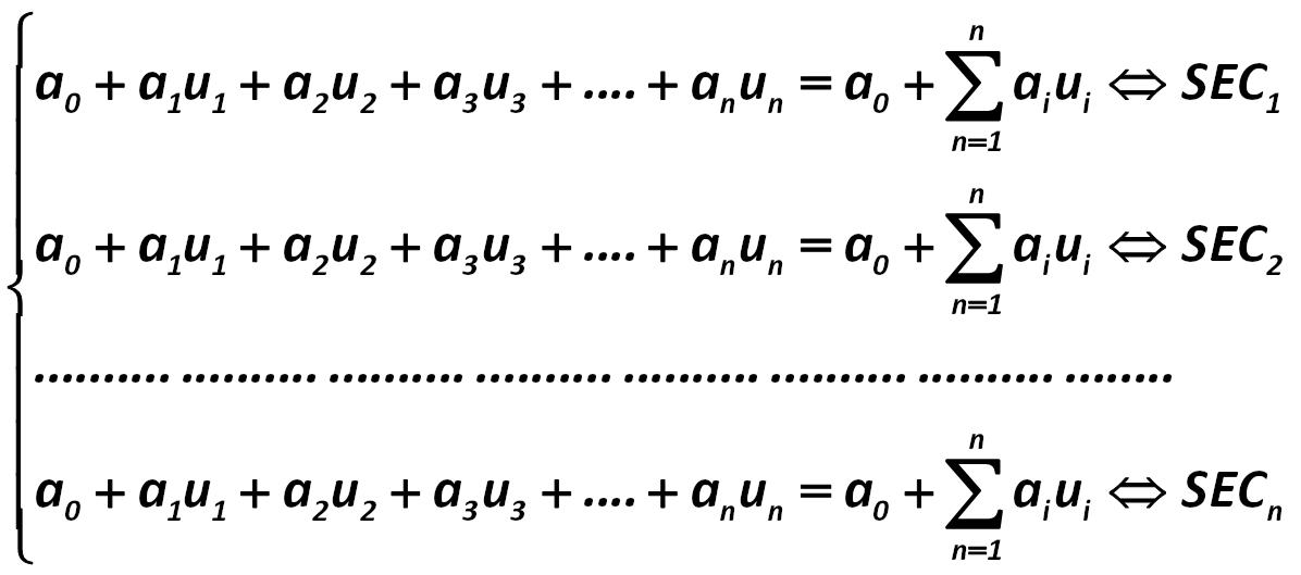
 The SEC index shows to which security portfolio corresponds each equation. Let us now compose and solve the system of equations for the JSC "Cobalt". Alexander Shemetev e13.jpg:1455x245, 50k |
 Then the average probable yield of the portfolio with minimum risk is: Alexander Shemetev e14.jpg:1455x142, 33k |
|
Then the portfolio risk for our example is: Alexander Shemetev e15.jpg:1462x117, 29k |
 Then the geometric middling of the yield of such security is: Alexander Shemetev e16.jpg:1536x348, 50k |
 The above calculation corresponds to the weighted approach to analysis of variance. For example, a standard measure of standard deviation for IE "N.I. Stella" will be the value: Alexander Shemetev e2.jpg:1208x176, 34k |
 Optimal portfolio is determined by the formula (262): Alexander Shemetev e262.jpg:756x74, 10k |
 Now, let's do the matrix multiplication in accordance with the formula (275): Alexander Shemetev e275.jpg:1675x450, 73k |
 Mathematical expectation of income in the next day will be: Alexander Shemetev e284.jpg:1250x137, 17k |
 So, for our IE "Stella" the value of standard deviation is: Alexander Shemetev e3.jpg:1095x185, 20k |
 In this example, the coefficient is equal to: Alexander Shemetev e4.jpg:487x131, 9k |
 So, if we optimize the portfolio by selling the asset number 1, then the company 1 has the opportunity to earn the following amount arbitrageurs : Alexander Shemetev e5.jpg:1510x285, 54k |
 We can verify this in the next calculation. Let JSC "Cobalt" to sell portfolio number 2. Then the arbitrage income is: Alexander Shemetev e6.jpg:1427x280, 53k |
|
This is the second version of the optimal portfolio; its arbitrageur is equal to: Alexander Shemetev e7.jpg:1235x84, 17k |
 Let us evaluate whether it is beneficial to sale the third portfolio: Alexander Shemetev e8.jpg:1406x284, 51k |
|
Arbitrageur of the third option of portfolio optimization is: Alexander Shemetev e9.jpg:1292x94, 17k |
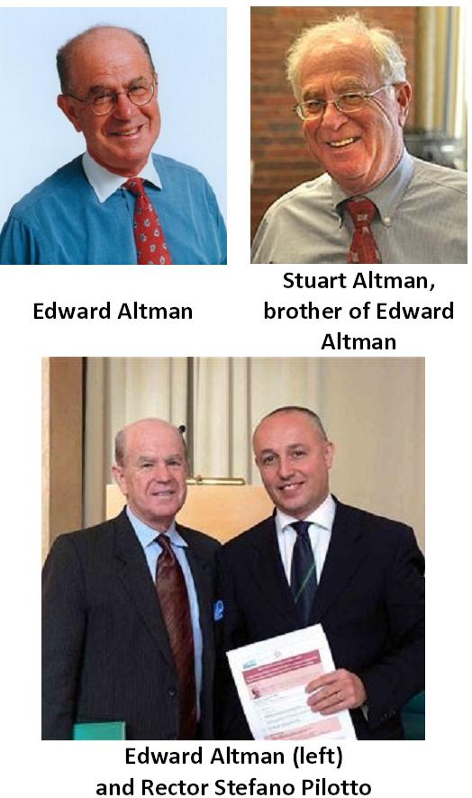 Edward Altman and Stuart Altman Edward Altman and Stuart Altman edward_and_stuart_altmans.jpg:524x886, 59k |
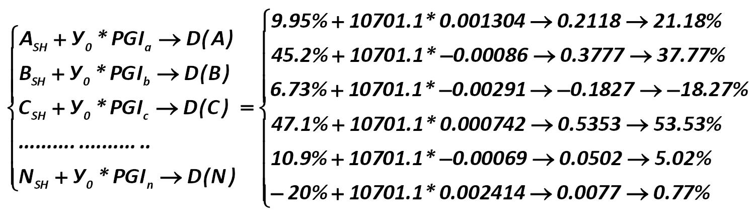
 For our example, this conversion rate will give the next most optimal for the investor portfolio: Alexander Shemetev epgi.jpg:1620x437, 79k |
 Professor Eva Kislingerova Eva Kislingerova eva_kislingerova.jpg:334x562, 24k |
 In our example, the Y0 index is equal to: Alexander Shemetev ey0.jpg:1605x243, 46k |
 Now we can calculate the optimal portfolio with a return of 5% from the system of equations (276): Alexander Shemetev ey1.jpg:1481x458, 92k |
 Y0 in this case will also change its form to: Alexander Shemetev ey2.jpg:1568x579, 95k |
 This Y0, in my opinion, more profoundly meets the current market conditions. Then the optimal portfolio of shares A – F has the next form: Alexander Shemetev ey3.jpg:1500x433, 93k |
 Gordon Springate Gordon Springate gordon_springate.jpg:305x411, 21k |
 Harry Markowitz Harry Markowitz harry_markowitz.jpg:604x447, 29k |
 Hatem Ben-Ameur and Pierre Rostan Hatem Ben-Ameur and Pierre Rostan hatem_ben_ameur_and_pierre_rostan.jpg:821x635, 56k |
|
The market researches stated the main production indicators for LLC "Luck" Alexander Shemetev ims0.jpg:894x26, 9k |
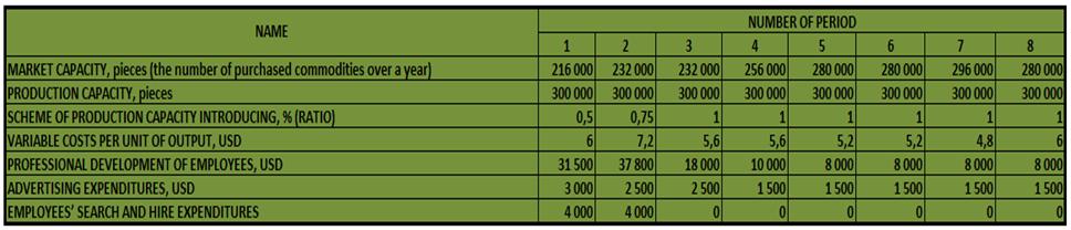 The market researches stated the main production indicators for LLC "Luck" Alexander Shemetev ims1.jpg:968x208, 43k |
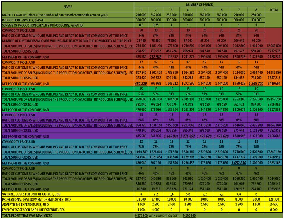 Analysis' results for LLC "Luck" Alexander Shemetev ims2.jpg:966x746, 191k |
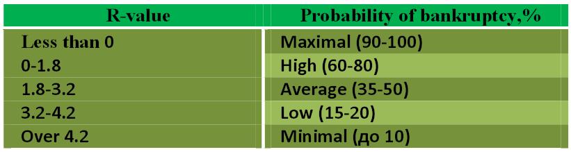 Ratio R values Baikal State University of Economics and Law, Irkutsk irkutsk_ratio.jpg:821x219, 29k |
 John Burr Williams John Burr Williams john_burr_williams.jpg:456x495, 19k |
 John Fulmer John Fulmer john_fulmer.jpg:368x425, 13k |
 The matrix system of forecasting bankruptcy on the model of William Henry Beaver, 1963 Alexander Shemetev m1.jpg:1508x463, 110k |
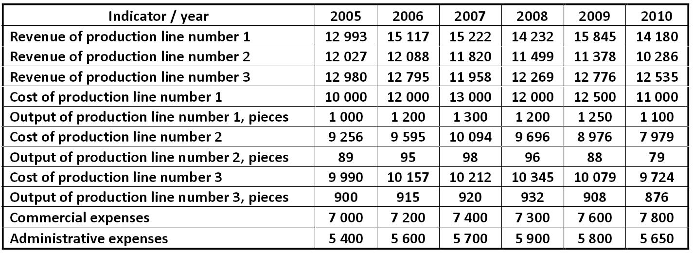 Table: Reported LLC "Dividend", millions USD Alexander Shemetev mt1.jpg:1425x522, 182k |
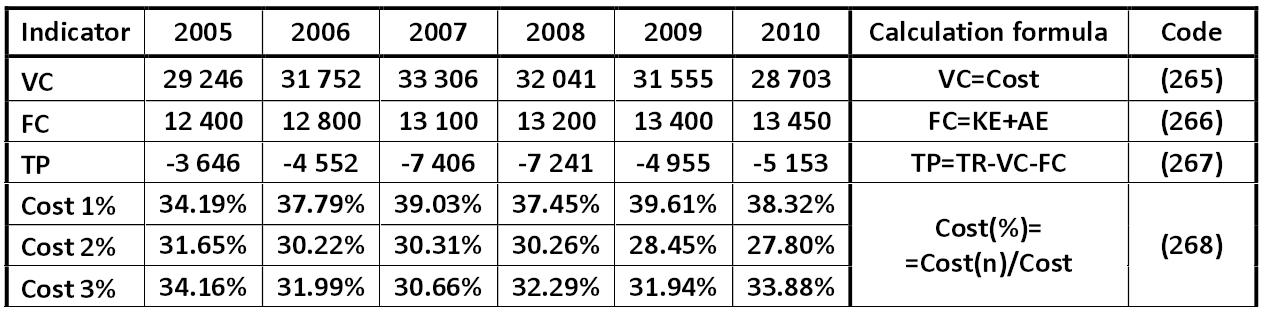 Table: Key marginal indicators of LLC "dividend", millions USD Alexander Shemetev mt2.jpg:1266x314, 93k |
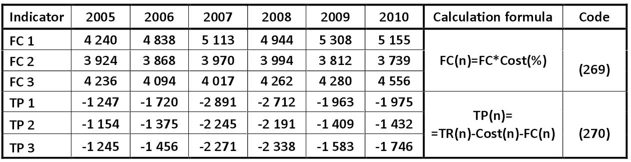 Table: Key marginal indicators of LLC "dividend", millions USD Alexander Shemetev mt3.jpg:1263x324, 80k |
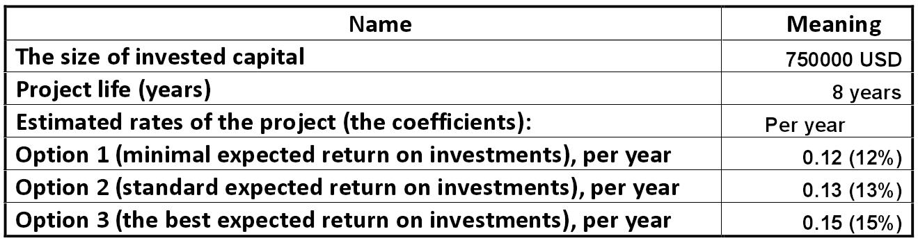 Table: Conditions on the investment project for LLC "Luck" Alexander Shemetev mt4.jpg:1319x350, 90k |
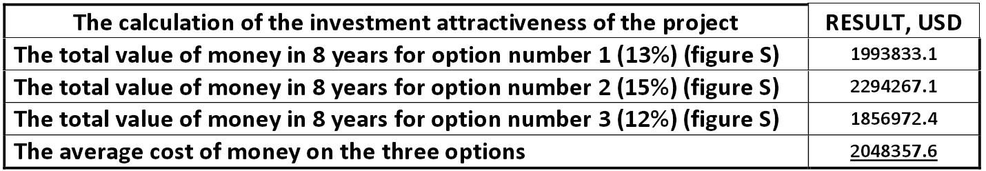 Table: Calculation of the investment attractiveness of the project Alexander Shemetev mt5.jpg:1430x248, 87k |
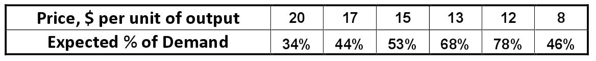 Table: Value for price and demand based on market research for company "Luck" Alexander Shemetev mt6.jpg:1168x120, 26k |
 Scheme: The general principle of neural networks in procedures of bankruptcy predicting Alexander Shemetev neyron1.jpg:1412x315, 25k |
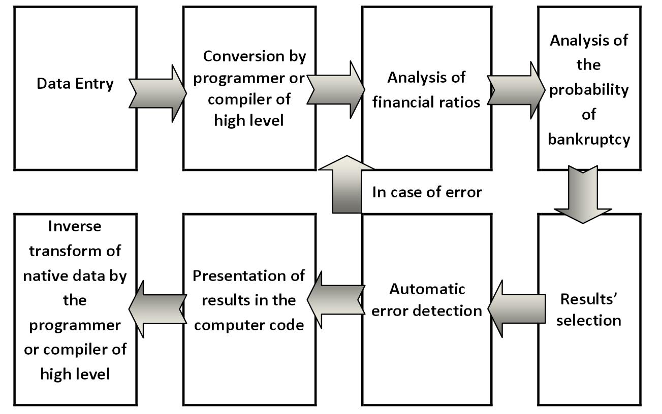 Scheme: A general algorithm of the method of neural networks Alexander Shemetev neyron2.jpg:1303x816, 100k |
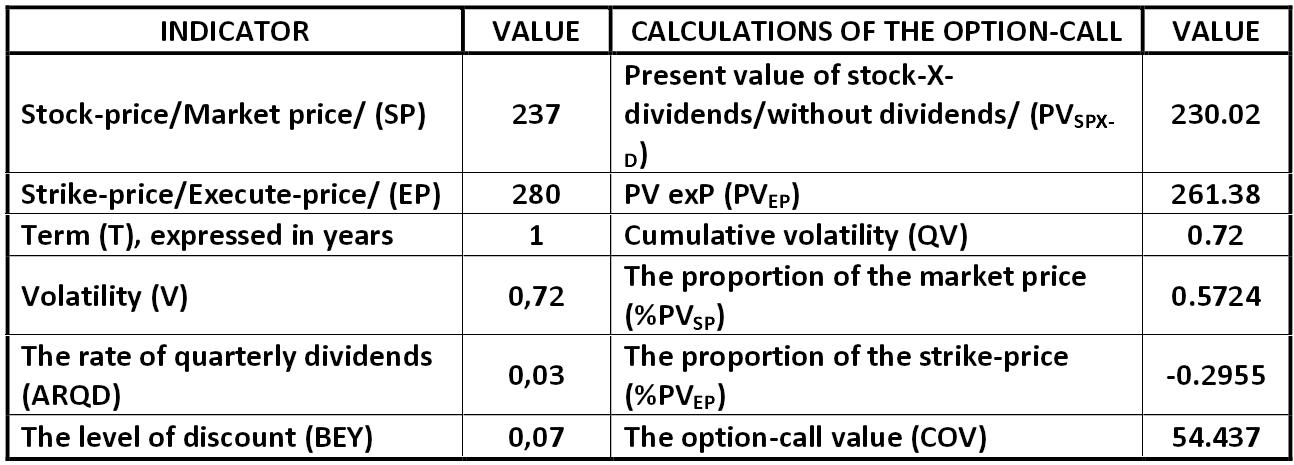 Table: Calculation of option-call value Alexander Shemetev ocv.jpg:1294x465, 112k |
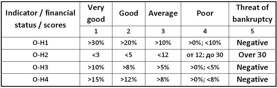 Matrix of Olejnik-Horvathova for bankruptcy predicting Silvia Horvathova and Pavol Olejnik ohm.jpg:907x290, 49k |
|
Average price symbol John Burr Williams price_average.jpg:42x52, 1k |
 px.jpg:87x51, 1k |
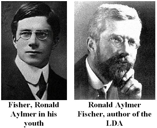 Ronald Aylmer Fisher Ronald Aylmer Fisher ra_fisher.jpg:544x445, 46k |
 Richard Taffler Richard Taffler richard_taffler.jpg:306x404, 14k |
 Chart: The yield / risk curve of portfolio Harry Markowitz s1.jpg:669x598, 73k |
 Diagram: Models for the prediction of bankruptcy by the Ooghe-Verbaere model: Alexander Shemetev s2.jpg:1303x512, 124k |
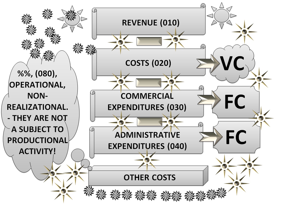 Scheme: Fixed and variable costs of any national reporting standard Alexander Shemetev s3.jpg:1150x834, 257k |
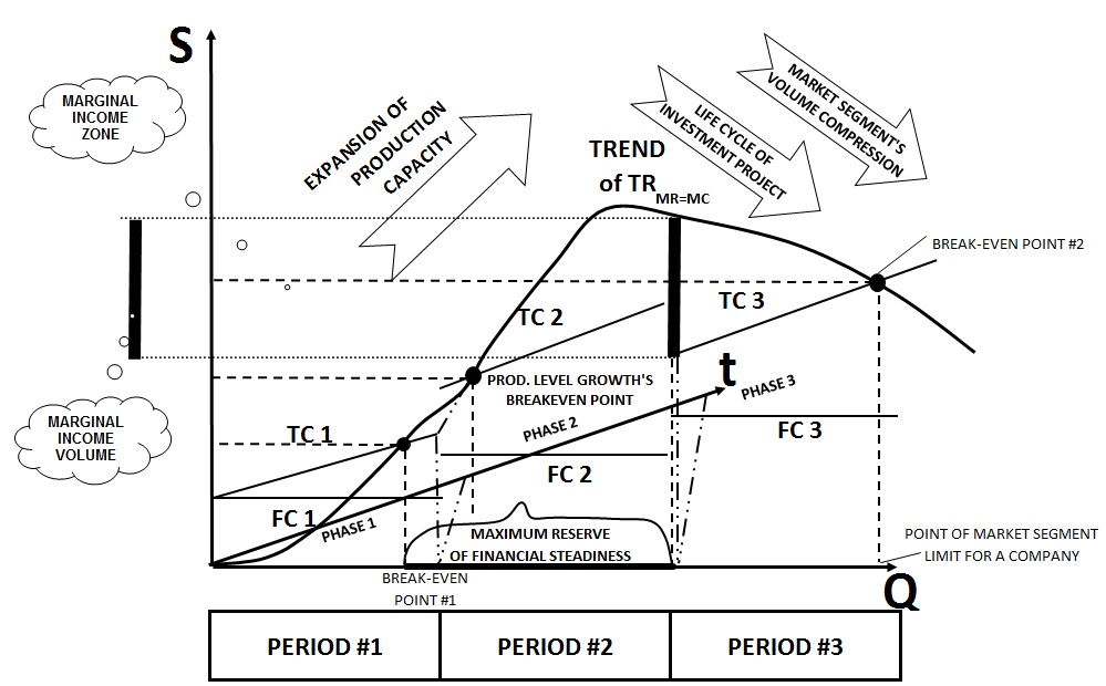 Schematic chart: The life cycle of the enterprise on the marginal model Alexander Shemetev s4.jpg:999x620, 140k |
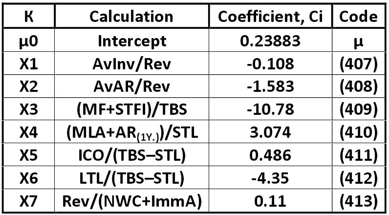 Table: Calculation of the first stage of the model Gibson-Stickney-Schroeder-Clark sgm.jpg:796x440, 75k |
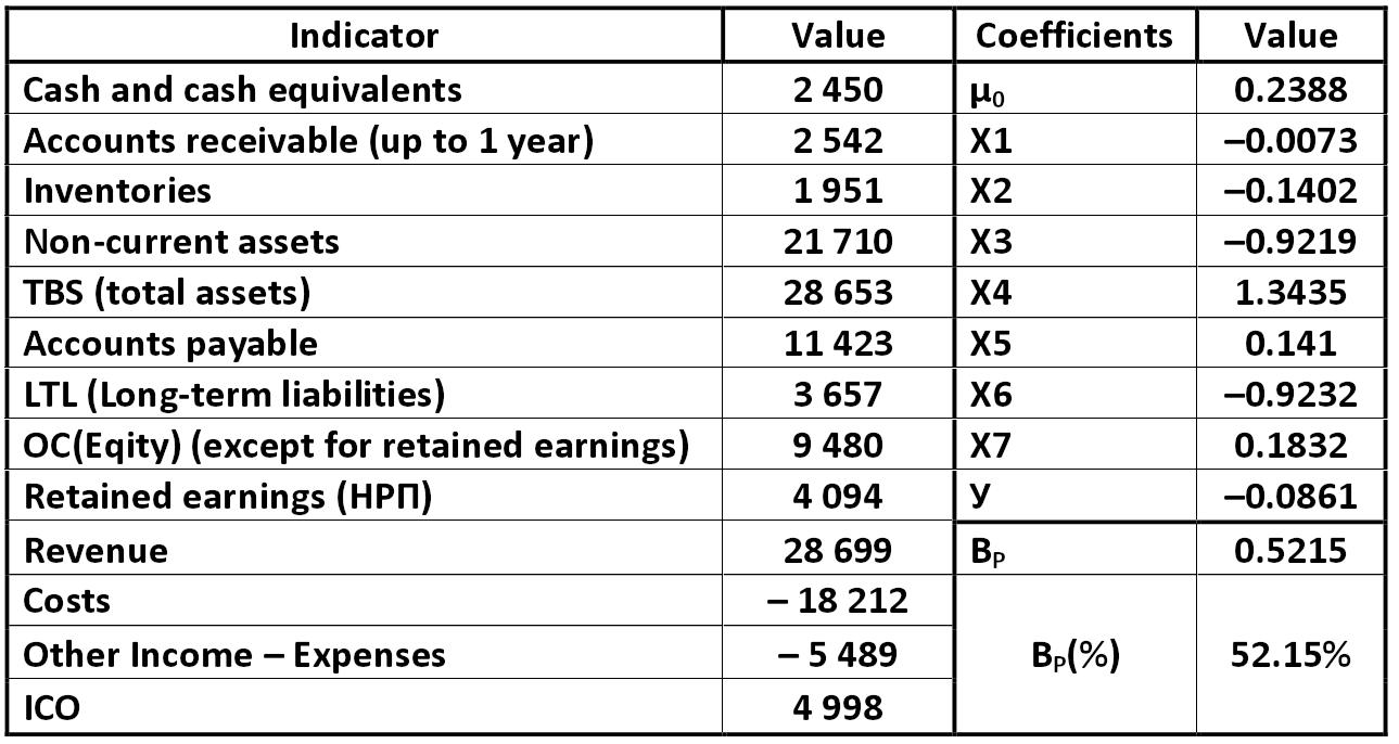 Table: Calculation of the probability of bankruptcy for the company "Stratum", thousand USD Alexander Shemetev sgm1.jpg:1289x686, 149k |
|
variation (classical and weight) Sir Francis Galton, Karl Pearson sigma.jpg:29x25, 0k |
 Stephen Alan Ross Stephen Alan Ross stephen_alan_ross.jpg:561x758, 34k |
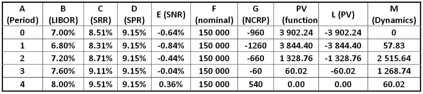 Table: Calculation of the SWAP by standard ED 162-B for a given scenario Alexander Shemetev swap.jpg:1421x318, 95k |
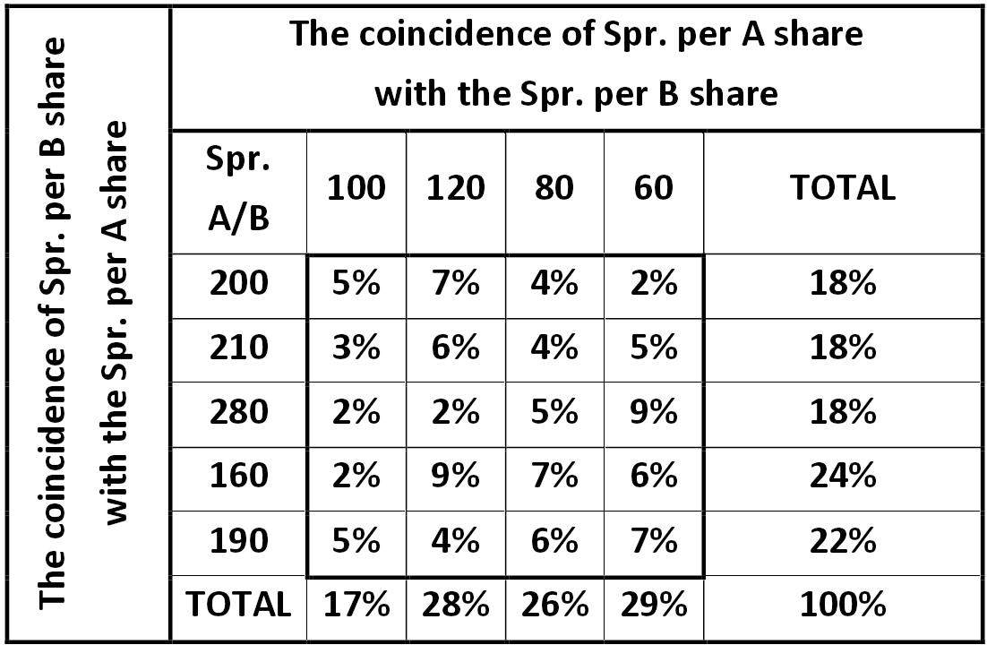 Covariate matrix of observations of stock prices of A and B Alexander Shemetev table1.jpg:1102x720, 111k |
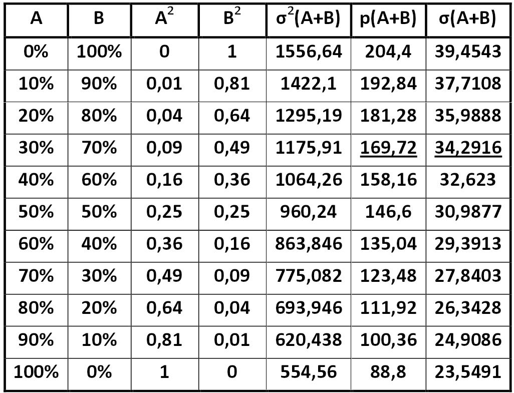 Matrix yield / risk of portfolio by Harry Markowitz for companies A and B Alexander Shemetev table2.jpg:1026x785, 155k |
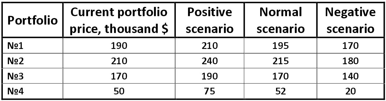 Table: Forecast value of the companies’ portfolios by the APT model Alexander Shemetev table3.jpg:1236x324, 65k |
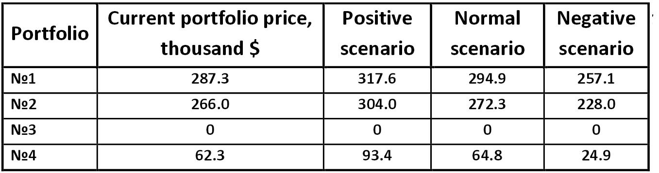 Table: Forecast value of the company's portfolio by the APT model Alexander Shemetev table4.jpg:1357x358, 75k |
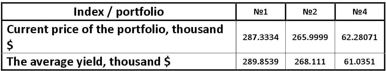 Table: Average price of the company JSC "Cobalt" portfolio by the APT model Alexander Shemetev table5.jpg:1288x239, 47k |
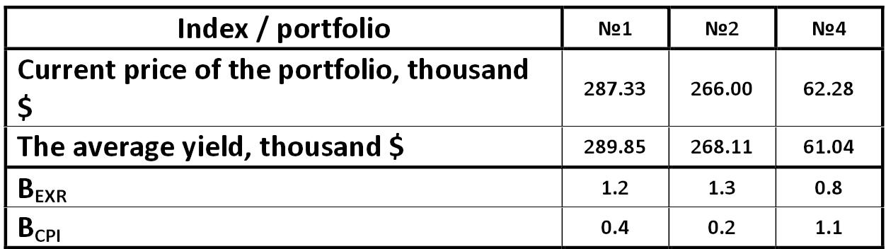 Table: The relationship between the indicatorial ? and portfolio course by the APT model Alexander Shemetev table6.jpg:1252x352, 55k |
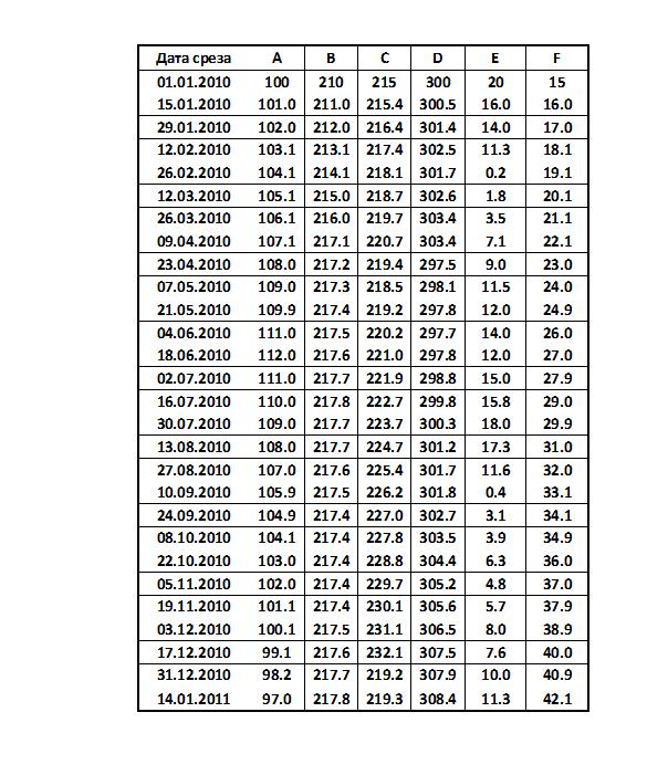 Table: Monitoring of the market shares of companies A – F from the beginning of 2010 to the beginning of 2011, USD Alexander Shemetev table7.jpg:585x701, 103k |
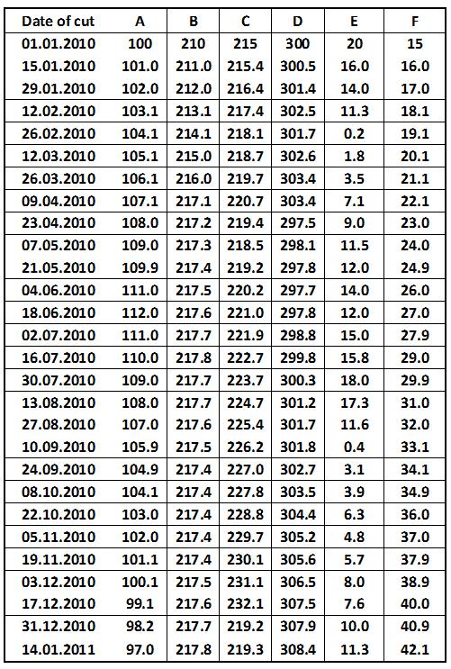 Table: Monitoring of the market shares of companies A – F from the beginning of 2010 to the beginning of 2011, USD Alexander Shemetev table7a.jpg:501x743, 130k |
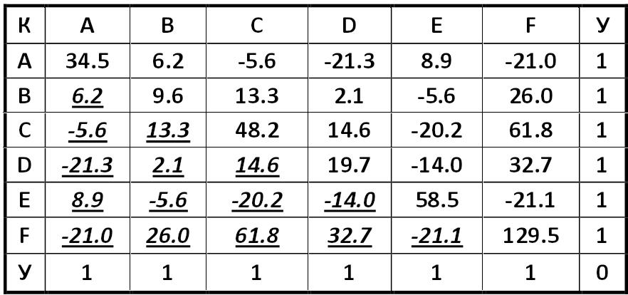 Covariance matrix system for companies A – F from the from the beginning of 2010 to the beginning of 2011 Alexander Shemetev table8.jpg:882x414, 66k |
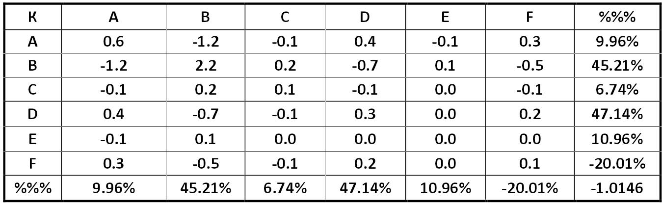 Covariance matrix system portfolio with minimal risk Alexander Shemetev table9.jpg:1349x414, 85k |
 The matrix system of forecasting of bankruptcy by the method of Ooghe- Verbaere Hubert Ooghe and Eric Verbaere tov.jpg:841x779, 248k |
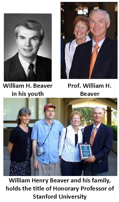 Prof. William H. Beaver Prof. William H. Beaver wh_beaver.jpg:499x847, 72k |
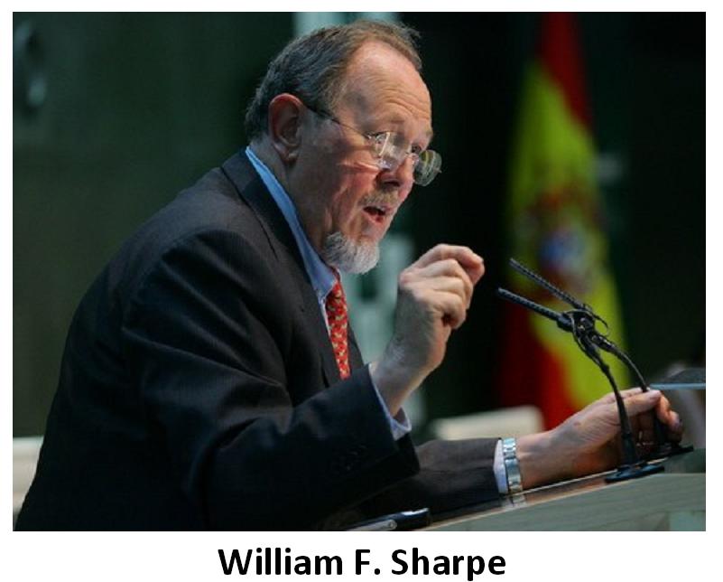 William F. Sharpe William F. Sharpe william_f_sharpe.jpg:801x644, 45k |
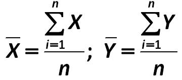
 X average Sir Francis Galton, Karl Pearson xav.jpg:52x50, 1k |
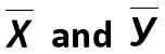 this is the average value of observed variables X and Y Sir Francis Galton xy.jpg:152x50, 2k |
|
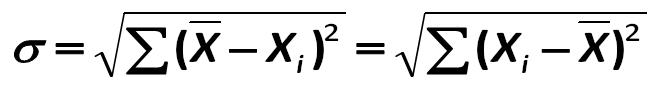
these are the standard deviations, which show the total amount that the value will be rejected averagely for any measure Sir Francis Galton xysigma.jpg:119x46, 1k |
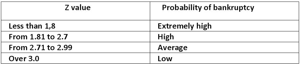 Table: The dependence of Z on the probability of bankruptcy Edward Altman z1.jpg:963x208, 30k |
|
Pointer (typographic sign) zzz1.jpg:45x26, 0k |
 Tick (typographical symbol) zzz2.jpg:77x67, 1k |
|
zzz3.jpg:27x25, 0k |