SECRETS OF NIKOLA TESLA
POTENTIAL ENERGY, CHARGES SEPARATION, GROUNDING AND PULSE EXCITATION
Vladimir Utkin u.v@bk.ru
INTRODUCTION
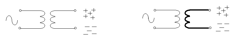
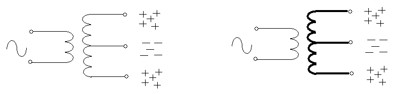
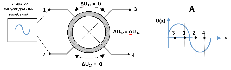
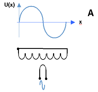
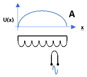
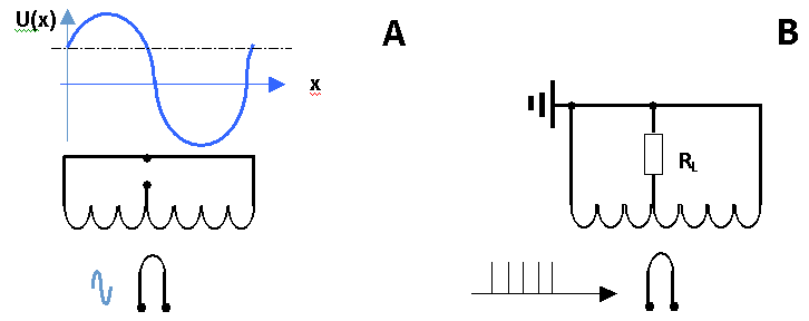
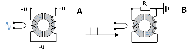
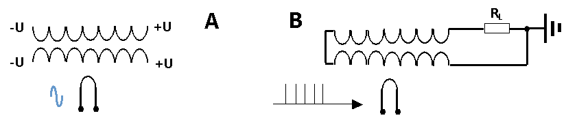
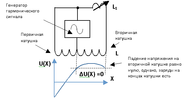
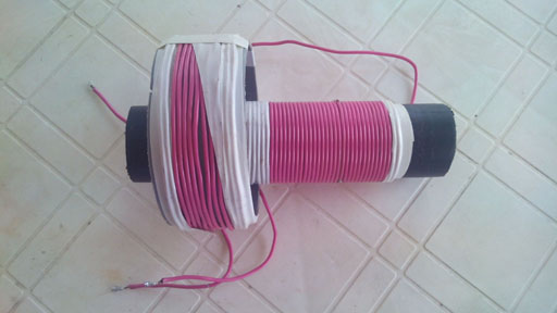
CHARGE SEPARATION: "ZERO-TRANSFORMER"
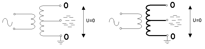
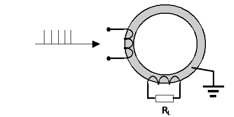
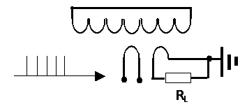
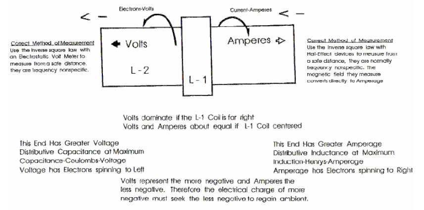
GROUNDING
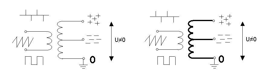
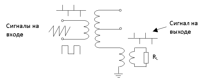
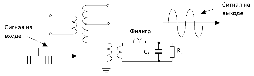
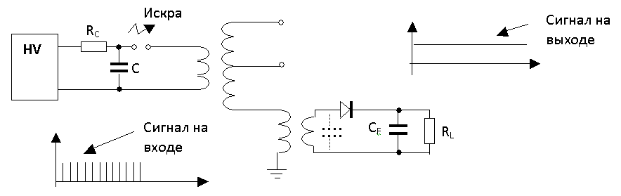
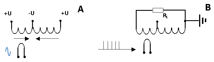
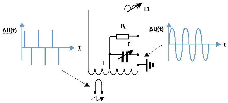
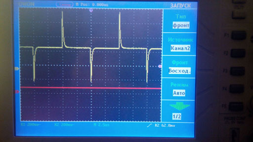
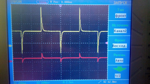
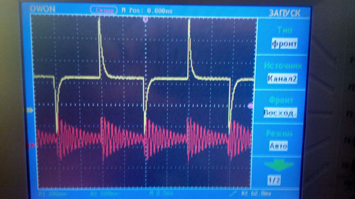
PULSE EXCITATION
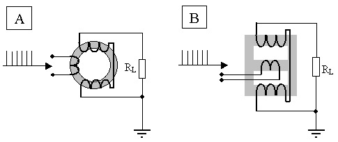
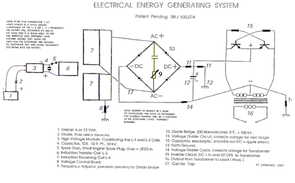
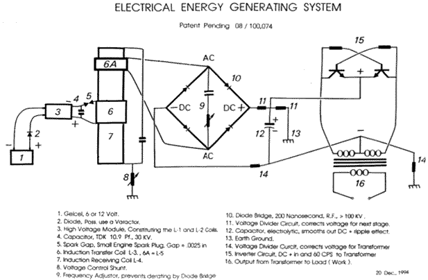
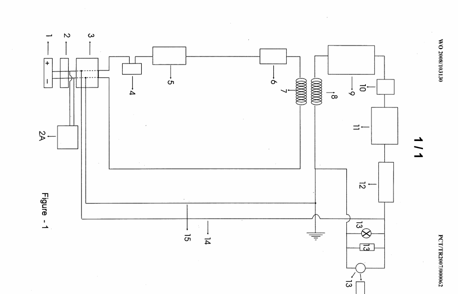
CONNECTION AND EXCITATION OPTIONS
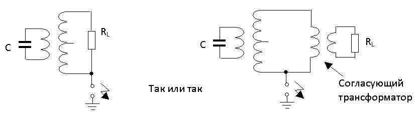
REVERSIBILITY "ZERO-TRANSFORMER"
THE PROBLEM OF VOLTAGE STABILIZATION
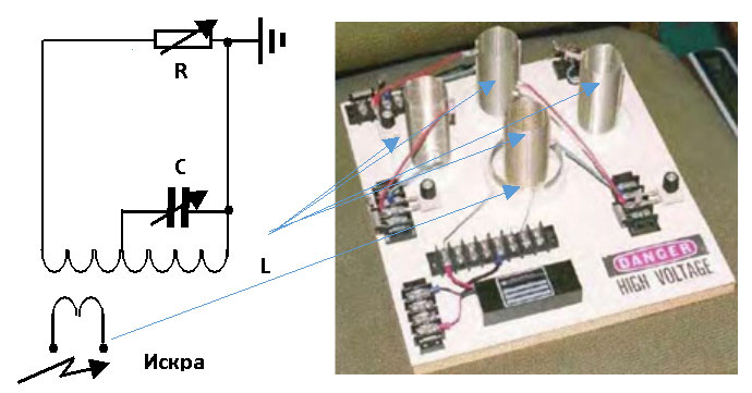
GROUNDING OF THE SECONDARY WINDING THROUGH A SPARK
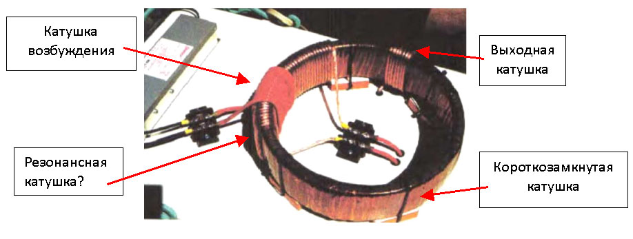
"ZERO-TRANSFORMER" ON SHORT-CIRCUITED COILS
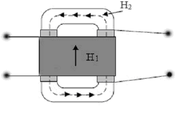
"ZERO-TRANSFORMER" ON A CLOSED MAGNETIC CIRCUIT
"ZERO-TRANSFORMER" WITH A COMPENSATING PART
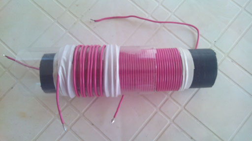
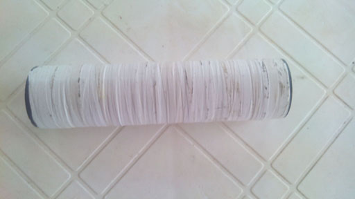
BIFILAR AS A " ZERO-TRANSFORMER"
WHAT DOES THE ENERGY IN THE LOAD DEPEND ON?
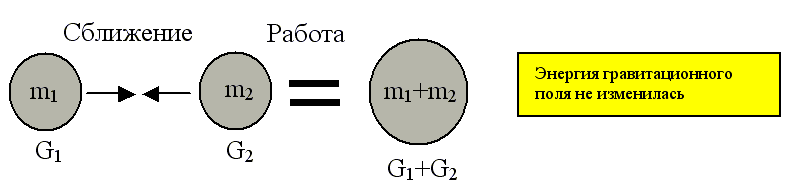
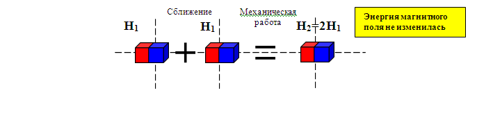
THE LAW OF CONSERVATION OF ENERGY
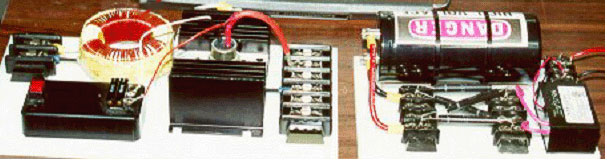
THE WORKS OF DONALD SMITH
WORKS BY TARIEL KAPANADZE
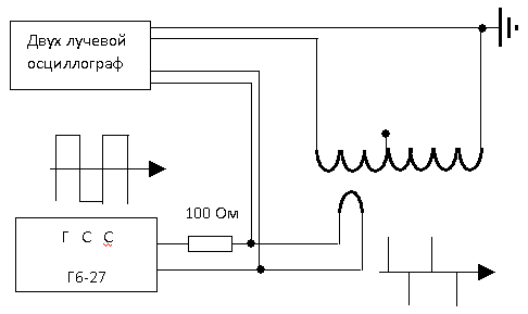
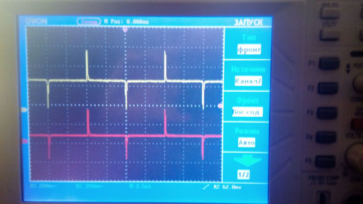
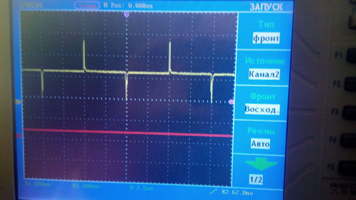
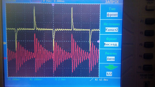
THE SIMPLEST EXPERIMENTS
"ZERO TRANSFORMER" WITH A COMPENSATING PART BASED ON FIG.18
GETTING THE FREQUENCY OF 50-60 HZ AT THE OUTPUT.